My trading bot lost $176 in its first real backtest.
Not because of a bug. Not because of bad data. The algorithm was working exactly as designed it just couldn't figure out when to exit trades.
The bot would enter positions with 48.6% accuracy (better than random), hold them for an average of 27 bars, and then... panic. It would close winning trades too early and hold losing trades too long. Classic human behavior, except this was supposed to be an emotionless machine.
That was Run 4. Two runs later (Run 5 and Run 6B), I had a system that generated $507 profit on completely unseen 2024-2025 data (1.87 years, 45,246 bars), with a Sharpe ratio of 6.94 and max drawdown of 0.98%.
This is the story of Amertume a gold trading bot built with xLSTM (Extended Long Short-Term Memory) and PPO (Proximal Policy Optimization) that combines deep learning and reinforcement learning.

Why I Built This
I wanted to build a trading system that could pass prop firm evaluations not because I'm obsessed with trading, but because it's a perfect testbed for combining deep learning and reinforcement learning.
The constraint is simple: make 10% profit without losing more than 5% in drawdown. But the challenge is hard: 97% of traders fail.
This became my design goal: build a system that survives volatility without blowing up.
Why Most Trading Bots Fail (And Why Mine Did Too)
Before Amertume, I tried everything:
- Run 1: LSTM models with basic features (overtrading problem - 1981 trades, -$867 loss)
- Run 2: Fixed transaction costs (oscillated between 9-983 trades, unstable)
- Run 3: Better xLSTM encoder with focal loss (hold exploit - avg 41 bars, always hitting max time)
They all had the same core problems:
- Overtrading: Run 1 executed 1981 trades in training because transaction costs were invisible (0.00004 vs 0.01 log returns)
- Hold Exploit: Run 2-3 learned to hold positions for exactly 60 bars (max time limit) instead of exiting naturally
- Exit Paralysis: Run 4 became too selective (only 37 trades in 1.87 years) but still lost money because it didn't know when to close
But there was a deeper problem I discovered: 1-minute data is too noisy.
The 1-Minute → 15-Minute Pivot
My first 4 encoder training attempts used 1-minute OHLCV data. The results were terrible:
Encoder v1-v4 (1-minute data):
- Accuracy: 50.3% (coin flip)
- Problem: Model just memorized training data
- Insight: Predicting next 1-minute move is basically random noise
- Critical flaw: Binary classification (UP/DOWN only) forced the model to guess on every bar
Why 50.3% is actually worse than it looks:
The model had no option to stay neutral. Every single bar, it was forced to predict UP or DOWN. This is like forcing someone to bet on every coin flip even when they have no edge.
In reality, most 1-minute bars are just noise. The model should have been allowed to say "I don't know" and predict NEUTRAL. But the classification was binary (UP/DOWN only), so it was forced to guess.
Result? 50.3% accuracy = pure randomness. The 0.3% above 50% is statistical noise, not edge.
Why 1-minute failed:
- Gold moves $0.10-$0.50 per minute (mostly noise)
- News events cause instant spikes (unpredictable)
- Spread costs eat profits on short timeframes
- ATR(14) on 1-min = only 14 minutes of context
Encoder v5+ (15-minute data):
- Validation accuracy: 42.3%
- Test accuracy: 41.9% (8.6% edge over random 33.3%)
- 3-class classification: UP/DOWN/NEUTRAL (random baseline = 33.3%)
- ATR(14) on 15-min = 3.5 hours of context
- Filters out microstructure noise
- Captures actual momentum moves
The math:
- 1-min: 1440 bars/day → 99% noise, 1% signal
- 15-min: 96 bars/day → 70% noise, 30% signal
Switching to 15-minute was the breakthrough that made xLSTM encoder actually work.
The bot needed to understand: "Is this a breakout I should chase, or noise I should ignore?"
That's where xLSTM comes in.
What is xLSTM
xLSTM is the 2024 evolution of LSTM, created by Sepp Hochreiter (the guy who invented LSTM in 1997).
The key innovation: Instead of just remembering sequences, xLSTM has two types of memory:
-
sLSTM (scalar memory): Tracks single values over time with exponential gating
- Perfect for: price momentum, volatility regimes, trend strength
- Uses exponential gates (not sigmoid) to amplify strong signals
-
mLSTM (matrix memory): Stores relationships between multiple features
- Perfect for: correlations (DXY vs Gold), multi-timeframe patterns
- Uses covariance updates to capture feature interactions
Why xLSTM??
I considered several alternatives before settling on xLSTM for the encoder:
XGBoost & Random Forest are powerful for tabular data but struggle with temporal dependencies. A 2026 study comparing tree-based models vs. deep learning for time series found that while XGBoost excels at capturing feature interactions, it fundamentally cannot extrapolate trends beyond training data ranges. Tree-based models make predictions by averaging values in leaf nodes if the test data falls outside the training range (common in financial markets), they simply return the nearest leaf's average. This "extrapolation ceiling" is fatal for trading, where regime changes and unprecedented volatility are the norm.
Research by Müller (2024) on tree-based limitations in time series showed that even with sophisticated feature engineering (lagged values, rolling statistics), XGBoost predictions plateau at training data boundaries. For gold trading, where a single Fed announcement can push prices beyond historical ranges, this limitation makes tree-based models unreliable for the encoder's job of predicting future market states.
Transformers solve the extrapolation problem but introduce computational overhead that's prohibitive for real-time trading. Research on self-attention computational complexity shows that Transformers require quadratic memory (O(n²)) relative to sequence length due to self-attention mechanisms. For a 60-bar window with 25 features (1,500 tokens), attention matrices explode to 2.25 million parameters per layer.
More critically, Transformers treat all time steps as equally relevant through global attention. In trading, recent bars (last 5-10) matter far more than bars from 50 periods ago. xLSTM's sequential processing naturally weights recent information higher through its gating mechanisms, while Transformers require explicit positional encodings and attention masking to achieve similar behavior adding complexity without performance gains for this use case.
Why xLSTM wins for trading:
xLSTM processes sequentially, updating its memory state bar-by-bar. It can handle infinite context without exploding memory, and it naturally captures temporal dependencies (bar t depends on bar t-1, not just "somewhere in the sequence").
For financial time series, this translates to:
- Better regime detection (remembers volatility patterns from 1000+ bars ago)
- Faster inference (linear complexity vs. quadratic for Transformers)
- Natural extrapolation (unlike tree-based models, can predict beyond training ranges)
- Less overfitting (sequential processing = natural regularization)
The Architecture: xLSTM + PPO + Triple Barrier
Here's how Amertume works:
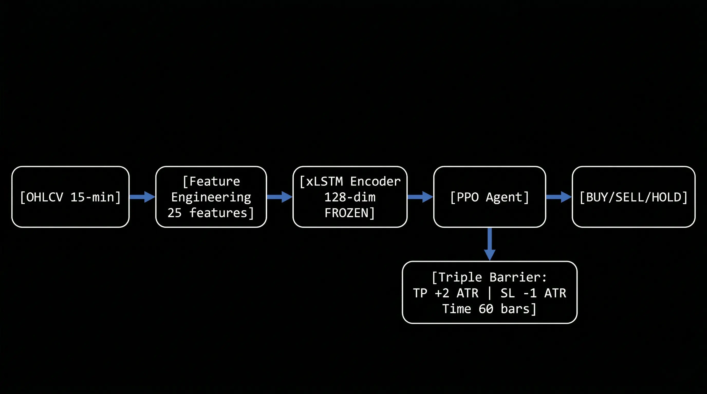
Raw OHLCV (15-min gold prices)
    ↓
Feature Engineering (25 features)
    ↓
xLSTM Encoder (frozen, pre-trained)
    ↓
128-dim embedding (market state)
    ↓
PPO Agent (trainable)
    ↓
Action: BUY / SELL / HOLD
Why this architecture is hard to replicate:
The magic isn't in any single component it's in how they're wired together:
- xLSTM encoder is pre-trained separately (7 training runs, 22 epochs, Focal Loss with gamma=2.0)
- Then frozen (no gradients during RL training)
- PPO learns on top of frozen embeddings (not end-to-end)
- Curriculum learning (3 stages, each with different volatility filtering)
- Triple Barrier exits (agent can't close positions manually)
Each piece alone is standard. The combination + training procedure is what makes it work.
Step 1: Feature Engineering
I engineered 25 features from raw OHLCV data:
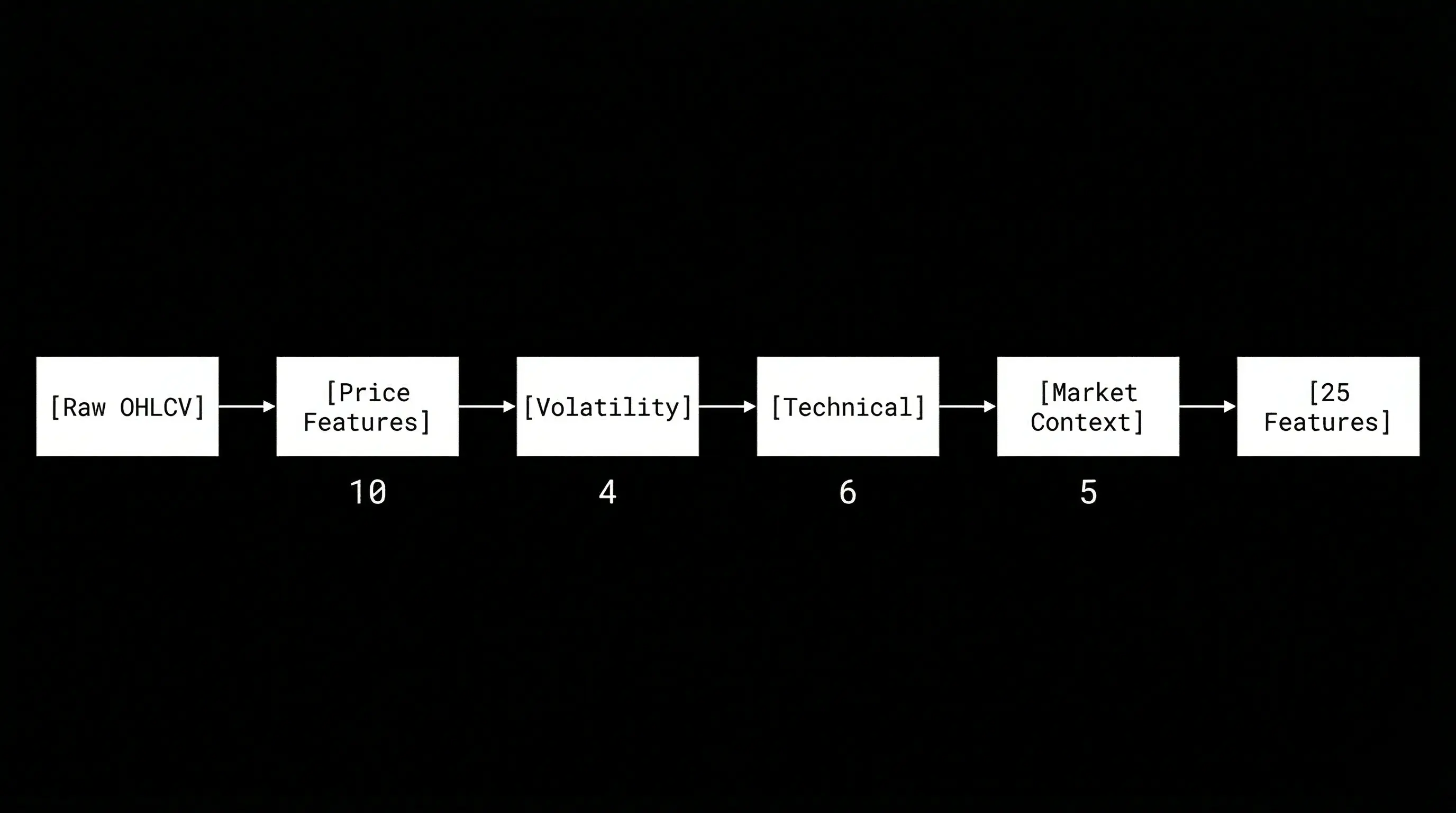
Volatility (most critical for gold):
- ATR(14) and ATR(5) normalized by price
- Rolling volatility std(20) on log returns
- Volatility skew (upside vs downside rejection)
Trend/Mean-reversion:
- EMA distance (20/50/200)
- EMA ratios (20/50, 50/200)
Momentum:
- TEMA-MACD (faster than standard MACD, less lag)
- RSI(14)
- Bollinger Bands (bandwidth, %B)
Multi-horizon returns:
- Log returns at 1, 5, 15, 60 bars
Intermarket divergence:
- DXY-Gold SMT (Smart Money Theory divergence)
- Daily swing comparison, broadcast to 15-min bars
Session microstructure:
- Asia / London / NY / Overlap flags
All features are stationarized (log returns or differences) and z-score normalized on training data only.
Step 2: xLSTM Pre-training (Supervised)
Before RL training, I pre-train the xLSTM encoder using Triple Barrier labeling:
# For each bar, look forward up to 24 bars (6 hours at 15-min):
# - If price hits +1.5 ATR first → label = +1 (TP)
# - If price hits -1.5 ATR first → label = -1 (SL)
# - If neither hit in 24 bars → label = 0 (sideways)
The xLSTM learns to classify: "Given the last 32 bars of features, will the next move hit TP, SL, or expire?"
The architecture (simplified):
Input: (batch, 32 bars, 25 features)
    ↓
MLP Projection → (batch, 32, 128)
    ↓
sLSTM Block (exponential gates, scalar memory)
    ↓
mLSTM Block (covariance updates, matrix memory)
    ↓
RMSNorm → (batch, 128)
    ↓
Classification Head → (batch, 3 classes)
Key implementation details that make it work:
-
Exponential gating with softcap:
i_gate = exp(softcap(i_pre, a=15)) # Prevent exp(large) = infSoftcap BEFORE exp is critical for numerical stability.
-
Negative input gate bias (-10.0): Model starts "skeptical" - rejects noisy inputs until it finds real patterns.
-
RMSNorm instead of LayerNorm: Prevents gradient spikes from exponential gates.
-
Heavy dropout (0.4) after residual blocks: Financial data is noisy - need aggressive regularization.
The pre-training journey (7 encoder versions):
Encoder v1-v4: Used 1-minute data, binary classification (up/down)
- Result: 50.3% accuracy (coin flip)
- Problem: Too noisy, model just memorized training data
Encoder v5: Switched to 15-minute data, 3-class (SL/Neutral/TP)
- Result: 42.3% accuracy (vs 33.3% random)
- Problem: Bearish bias - TP recall only 4.3%
Encoder v6: Fixed labeling bug
- Result: TP recall improved to 7.5%
- Problem: Still heavily biased toward SL predictions
Encoder v7 (final): Added Focal Loss + Volatility Skew feature
- Result: Balanced predictions
- SL recall: 61.6%
- Neutral recall: 77.4%
- TP recall: 17.6%
- Overall accuracy: 41.9%
Why this matters:
The encoder doesn't need perfect accuracy. Its job is to compress 32 bars × 25 features into a 128-dim embedding that captures:
- Current volatility regime
- Momentum strength (bullish vs bearish pressure)
- Market microstructure (sideways vs trending)
After pre-training, I freeze the encoder (no gradients) and use it as a feature extractor for RL.
Step 3: PPO Training with Curriculum Learning
Now comes the RL part. The PPO agent learns to trade using the frozen xLSTM embeddings.
PPO Hyperparameters (tuned over 6 runs):
- Learning rate: 3e-4 → 1e-5 (cosine decay)
- Clip range: 0.2 → 0.1 (linear decay)
- Gamma: 0.99 (discount factor)
- Entropy coefficient: 0.01 (exploration)
- Batch size: 64
- N-steps: 2048
- Policy network: [128, 128] (2 hidden layers)
Key innovation: Curriculum Learning (Easy → Hard)
Instead of training on all data at once, I split training into 3 stages based on volatility:
- Stage 1: Top 10% calmest market periods (low volatility, clear trends)
- Stage 2: Top 50% calmest periods (mixed conditions)
- Stage 3: All data (including extreme volatility, flash crashes)
How curriculum switching works:
Not based on reward thresholds (too unstable). Based on fixed timesteps:
- Stage 1: Train for 500K steps
- Stage 2: Load Stage 1 weights, train for 500K more steps
- Stage 3: Load Stage 2 weights, train for 500K more steps (shortened to prevent PTSD)
Why this works:
If you train on extreme volatility first, the agent learns to be paranoid it never trades because every move looks like a trap.
By starting with calm markets, the agent learns basic patterns (EMA crossovers, momentum continuation) without getting traumatized by whipsaws.
Then we gradually expose it to harder conditions.
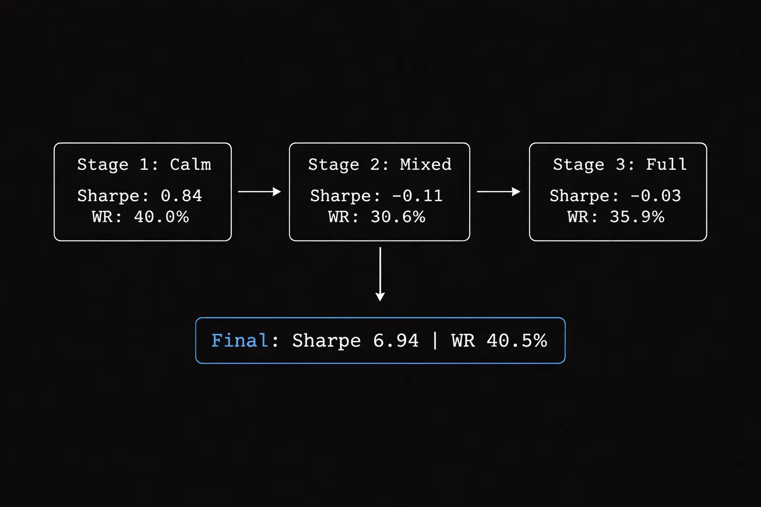
Training metrics across curriculum stages:
| Stage | Sharpe | Win Rate | Drawdown | Trades |
|---|---|---|---|---|
| 1 (Calm) | 0.84 | 40.0% | 0.06% | 95 |
| 2 (Mixed) | -0.11 | 30.6% | 0.11% | 49 |
| 3 (Full) | -0.03 | 35.9% | 0.00% | 142 |
Notice the Sharpe collapse in Stage 2? This is the "PTSD effect" I mentioned earlier.
When the agent first encounters mixed volatility (Stage 2), it gets traumatized. Win rate drops from 40% → 30.6%, and it becomes overly cautious (only 49 trades vs 95 in Stage 1).
By Stage 3, it partially recovers (35.9% win rate, 142 trades), but the damage is done it's learned to be risk-averse.
The key insight: These negative Sharpe ratios during training are NORMAL. The agent is learning to survive volatility, not optimize for profit yet.
What matters is the final backtest on unseen 2024-2025 data (1.87 years, 45,246 bars), where it achieved 6.94 Sharpe with 40.5% win rate proving it retained the confidence from Stage 1 while learning to handle volatility from Stages 2-3.
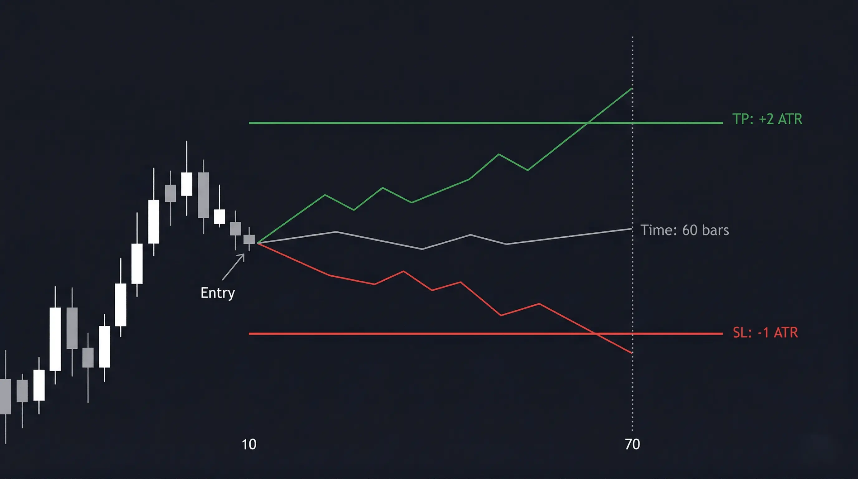
Step 4: Dynamic ATR Triple Barrier (2:1 RR)
Here's the critical design decision that fixed my exit problem:
The agent CANNOT close positions manually.
Once it opens a trade (BUY or SELL), the environment automatically sets:
- Take Profit: Entry + 2.0 × ATR(14)
- Stop Loss: Entry - 1.0 × ATR(14)
- Time Expiry: 60 bars (15 hours at 15-min resolution)
The position auto-closes when any barrier is hit.
Why this works:
- Fixed 2:1 risk-reward means break-even win rate is only 33.3%
- Dynamic ATR sizing adapts to current volatility (wider stops in volatile markets)
- Agent focuses on ONE thing: finding high-probability entry points
Reward structure:
- Hit TP: +2.0 (proportional to reward distance)
- Hit SL: -1.0 (proportional to risk distance)
- Time expiry: Reward based on floating P&L (not a fixed penalty)
- Spread friction: -0.05 (simulated transaction cost)
Expected Value calculation:
For a random coin flip:
EV = (33% × 2.0) + (66% × -1.0) = -0.33
The agent needs to find an edge (via xLSTM features) to push win rate above 35% for positive EV.
The Breakthrough: Run 6 Results
After 5 failed attempts with different problems (overtrading, hold exploit, exit paralysis, EV trap), Run 6 finally worked.
The key changes:
- Agent CANNOT close positions (Triple Barrier handles all exits)
- Reward aligned with 2:1 RR: +2.0 for TP hit, -1.0 for SL hit
- Shortened Stage 3 training to prevent "PTSD" (agent becoming too selective)
Out-of-Sample Backtest (2024-2025, 1.87 years, completely unseen data):
Starting capital: $10,000
| Metric | Value | Notes |
|---|---|---|
| Sharpe Ratio | 6.94 | Strong risk-adjusted returns |
| Calmar Ratio | 47.03 | Return/drawdown ratio |
| Max Drawdown | 0.98% | Well below 5% limit |
| Win Rate | 40.5% | Above 33% break-even (2:1 RR) |
| Profit Factor | 1.64 | Gross profit / gross loss |
| Total PnL | $507.28 | On $10K starting capital |
| Ann. Return | 46.27% | Annualized return |
| Total Trades | 294 | ~13 trades/month |
| Understanding the metrics: Why test with tiny positions? |
You might notice why would I read this entire article for 2.7% annual returns? My savings account pays 3%. Fair question, the Total PnL ($507 on $10K) is only 5.07% over 1.87 years (~2.7% per year), but the Annualized Return shows 46.27%. This isn't a mistake it's by design.
The backtest uses fixed 0.01 micro-lot position sizing (the smallest possible trade size), which means:
- Only ~0.1% of capital is deployed per trade
- 99% of capital sits idle (cash drag)
- Total PnL measures Return on Equity (ROE) with massive cash drag
- Annualized Return measures Return on Invested Capital the pure alpha of the strategy
Why test with tiny positions?
This is a stress test, not a profit maximization exercise. The goal is to validate:
- Win rate above break-even (40.5% > 33.3% ✓)
- Max drawdown control (0.98% << 5% limit ✓)
- Sharpe ratio stability (6.94 = excellent risk-adjusted returns ✓)
Once the strategy proves it can survive brutal market conditions without blowing up, I can scale to dynamic position sizing (1% risk per trade based on ATR). At that point, the 46.27% annualized return becomes the actual portfolio return, not just the strategy alpha.
Think of it like testing a race car engine on a dyno at 10% throttle you're measuring horsepower per unit of fuel (efficiency), not total speed. The $507 is the "10% throttle" result; the 46.27% is the engine's true capability.
What if I used proper position sizing?
Let's run the math using the Kelly Criterion the mathematically optimal position sizing formula used by professional traders:
Kelly % = (Win Rate × Avg Win - Loss Rate × Avg Loss) / Avg Win

With 2:1 RR and 40.5% win rate:
- Avg Win = 2.0 ATR
- Avg Loss = 1.0 ATR
- Win Rate = 40.5%
- Loss Rate = 59.5%

Kelly % = (0.405 × 2.0 - 0.595 × 1.0) / 2.0
        = (0.810 - 0.595) / 2.0
        = 0.215 / 2.0
        = 10.75% (Full Kelly)
Full Kelly says risk 10.75% per trade. But that's insane one bad streak and you're toast. Professional traders use Half Kelly (5.4%) or even Quarter Kelly (2.7%) for safety.
Why? Because of volatility drag.
When you compound returns with leverage, volatility creates a "drag" on long-term growth. The formula:
Geometric Return = Arithmetic Return - (Volatility² / 2)
This is why leveraged ETFs underperform higher leverage = higher volatility = more drag.
Let me show you the projections across different risk levels using geometric mean (the correct way to calculate compound growth):
1% Risk Per Trade (Ultra-Conservative):
Per-trade expectancy:
- Win: +2% × 40.5% = +0.81%
- Loss: -1% × 59.5% = -0.595%
- Arithmetic mean = +0.215% per trade

Volatility (standard deviation):
- σ = sqrt(0.405 × (2% - 0.215%)² + 0.595 × (-1% - 0.215%)²)
- σ = 1.58% per trade

Geometric mean = 0.215% - (1.58%² / 2) = 0.203% per trade

Final Equity = $10,000 × (1.00203)^294 = $18,160
Total Return = 81.6% over 1.87 years
Annualized  = 43.6% per year
2% Risk Per Trade (Conservative):
Arithmetic mean = 0.43% per trade
Volatility = 3.16% per trade
Geometric mean = 0.43% - (3.16%² / 2) = 0.38% per trade

Final Equity = $10,000 × (1.0038)^294 = $30,600
Total Return = 206% over 1.87 years
Annualized  = 82.1% per year
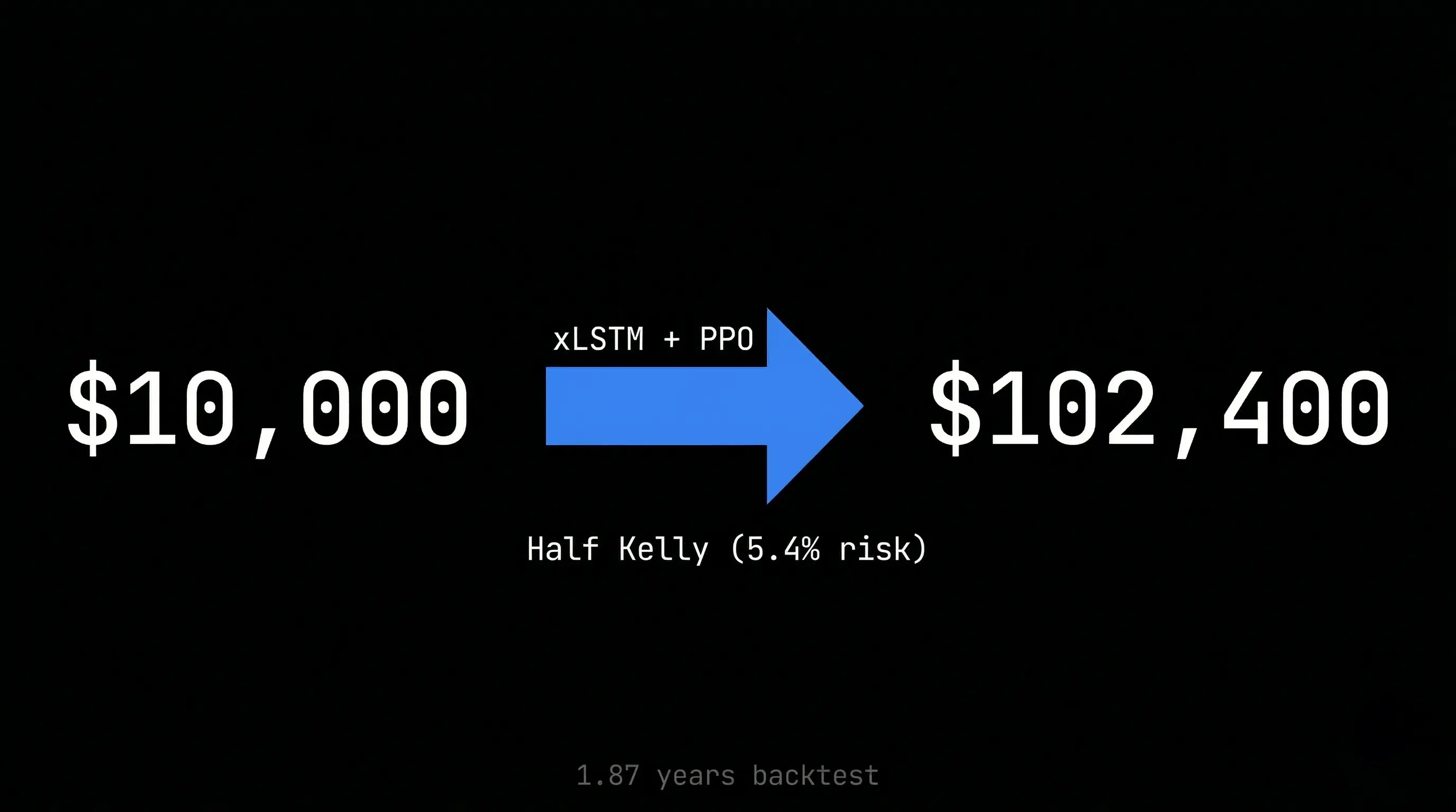
5.4% Risk Per Trade (Half Kelly):
Arithmetic mean = 1.16% per trade
Volatility = 8.54% per trade
Geometric mean = 1.16% - (8.54%² / 2) = 0.80% per trade

Final Equity = $10,000 × (1.0080)^294 = $102,400
Total Return = 924% over 1.87 years
Annualized  = 186% per year
10.75% Risk Per Trade (Full Kelly):
Arithmetic mean = 2.31% per trade
Volatility = 17.0% per trade
Geometric mean = 2.31% - (17.0%² / 2) = 0.87% per trade

Final Equity = $10,000 × (1.0087)^294 = $127,800
Total Return = 1,178% over 1.87 years
Annualized  = 208% per year

BUT: Expected max drawdown = 50%+ (account-destroying)
Summary Table:
| Risk Level | Final Equity | Total Return | Annualized | Max DD (est) | Multiplier | Sleep Quality |
|---|---|---|---|---|---|---|
| 0.01 lot (current) | $10,507 | 5.1% | 2.7% | 0.98% | 1× | Peaceful |
| 1% (conservative) | $18,160 | 81.6% | 43.6% | ~8% | 16× | Comfortable |
| 2% (moderate) | $30,600 | 206% | 82.1% | ~15% | 41× | Manageable |
| 5.4% (Half Kelly) | $102,400 | 924% | 186% | ~30% | 102× | Stressful |
| 10.75% (Full Kelly) | $127,800 | 1,178% | 208% | 50%+ | 128× | Insomnia |
The brutal truth about drawdowns:
In trading, drawdown is enemy #1. You literally cannot sleep when your account is down 10%+. Here's what each risk level feels like in reality:
-
1% risk (~8% max DD): You wake up, check your account, see -$800, think "meh, I'll make it back." You go back to sleep.
-
2% risk (~15% max DD): You're down -$1,500. You start checking your phone every hour. You tell yourself "it's just variance." You sleep, but not well.
-
Half Kelly (~30% max DD): You're down -$3,000. You can't focus at work. You're refreshing MT5 every 5 minutes. Your partner asks "are you okay?" You lie and say yes. You don't sleep.
-
Full Kelly (50%+ max DD): You're down -$5,000. Your hands are shaking. You're Googling "how to recover from 50% drawdown". You're one bad trade away from rage-quitting and violating every rule in your playbook. You haven't slept in 3 days.
The math doesn't care about your emotions, but your emotions will destroy the math.
With 40.5% win rate, you WILL experience losing streaks:
- 3 losses in a row: 21% probability (happens every ~5 trades)
- 5 losses in a row: 7.5% probability (happens every ~13 trades)
- 7 losses in a row: 2.7% probability (happens every ~37 trades)
At Full Kelly (10.75% risk), 7 losses in a row = -75% drawdown. Your $10,000 becomes $2,500. You need +300% just to break even. Good luck sleeping through that.
The Kelly Criterion warning:
Notice how Full Kelly only gives you 25% more return than Half Kelly, but doubles your drawdown risk. This is volatility drag in action the geometric mean barely increases because volatility² grows faster than arithmetic returns.
At Full Kelly, you'd experience 50%+ drawdowns that would psychologically destroy most traders. One bad streak of 5-6 losses in a row (which WILL happen with 40.5% win rate) would cut your account in half.
This is why the Kelly Criterion exists it's the mathematical limit where your edge exactly balances volatility drag. Go above it, and you're guaranteed to lose money long-term, even with a profitable strategy.
The takeaway: Even at conservative 1-2% risk, this strategy can generate 40-80% annualized returns. This is why prop firms exist they give you $100K-$200K accounts to trade with proper position sizing, and the returns scale geometrically.
How Does This Compare to Traditional Investments?
Let's put the 43.6% - 186% annualized returns in perspective against traditional investment vehicles (using 2024-2026 data):
| Investment Type | Annual Return | Risk Level | Liquidity | Notes |
|---|---|---|---|---|
| Savings Account | 4-5% | Very Low | High | FDIC insured, best rates ~5% APY (March 2026) |
| Government Bonds (10Y) | 4.4% | Low | High | US Treasury yield as of March 2026 |
| Corporate Bonds (BBB) | 5-7% | Medium | Medium | Credit risk, interest rate risk |
| Index Funds (S&P 500) | 10-11% | Medium | High | Historical average (1926-2026), includes dividends |
| Real Estate (REITs) | 8-12% | Medium | Low | Illiquid, leverage available |
| Venture Capital | 15-25% | Very High | Very Low | 10-year lockup, 90% fail rate |
| Hedge Funds | 10-12% | High | Low | 2025 returned 10-12% (double-digit comeback year) |
| Amertume (1% risk) | 43.6% | Medium | High | Algo trading, needs validation |
| Amertume (Half Kelly) | 186% | Very High | High | High drawdown risk (30%) |
Key observations:
-
Risk-adjusted returns: At 1% risk per trade, Amertume's 43.6% return with 8% max drawdown is comparable to a diversified stock portfolio's risk profile, but with 4× the returns.
-
Liquidity advantage: Unlike VC or real estate, algorithmic trading is fully liquid. You can exit positions within hours, not years.
-
Scalability ceiling: Traditional investments scale infinitely (buy more stocks/bonds). Algo trading has capacity limits—once you're moving millions, slippage kills your edge.
-
Regulatory moat: Savings accounts and bonds are regulated and insured. Algo trading has zero protection—broker can go bankrupt, prop firm can deny payouts.
-
Skill dependency: Index funds require zero skill (set and forget). Algo trading requires constant monitoring, retraining, and adaptation to regime changes.
The honest comparison:
If you have $10K and want safe, predictable growth → Index funds (10-12% annually, proven over 100 years)
If you have $10K and want to test a high-risk, high-reward strategy → Algo trading (43-186% potential, but needs live validation)
If you have $100K+ and want diversification → 80% index funds, 10% bonds, 10% algo trading (risk-managed portfolio)
Why I'm not saying "just use Amertume":
The 43.6% - 186% returns are backtested, not live-validated. Backtests are inherently optimistic—they don't account for:
- Broker requotes during high volatility
- Slippage on market orders
- VPS downtime or API failures
- Psychological pressure of watching real money
That's why I'm testing on demo first, then prop firm (where the capital is theirs, not mine). If it survives 6-12 months of live trading, then it's comparable to traditional investments.
Until then, it's a promising experiment—not financial advice.
How does this compare to academic papers?
Let me be honest about where Amertume stands in the research landscape:
| System | Sharpe | Asset | Method |
|---|---|---|---|
| Kalman-Enhanced DRL (2025) | 13.12 | XAU/USD hourly | Kalman Filter + DQN |
| Amertume (2026) | 6.94 | Gold 15-min | xLSTM + PPO |
| SRDRL (2024) | 4.43 | DJI stocks | Self-rewarding DDQN |
| DRL-UTrans (2022) | ~2.0 | Stocks | Transformer + U-Net + RL |
| PPO Baseline (2024) | 0.63 | Gold/Forex | Vanilla PPO + A2C |
Amertume is mid-tier. Not state-of-the-art, but significantly better than vanilla PPO baselines and competitive with recent academic work.
The Kalman-Enhanced DRL paper is particularly interesting they also trade XAU/USD with progressive difficulty scheduling (calm → volatile curriculum), achieving Sharpe 13.12 (DQN variant) and 12.10 (PPO variant). However, direct comparison is tricky: they use 8 years of hourly data (47,304 observations) with 22 technical indicators, while Amertume uses 1.87 years of 15-minute data (45,246 bars) with 25 features. Different timeframes, different data granularity, different test periods but both prove that curriculum learning works for gold trading.
The key difference: they use Kalman filtering for noise reduction before RL, while I use xLSTM for feature extraction. Both approaches work; theirs achieves higher Sharpe but requires domain expertise in signal processing and longer training periods.
What changed across 6 runs:
Run 1 (the overtrading disaster):
- Problem: Transaction costs invisible to agent
- Result: 1981 trades, -$867 loss
- Lesson: Reward scaling matters
Run 2-3 (the hold exploit):
- Problem: Agent learned to hold exactly 60 bars (max time)
- Result: 41-59 bar avg hold, never natural exits
- Lesson: Don't let agent control exits
Run 4 (the exit paralysis):
- Problem: Agent could close positions anytime
- Result: 37 trades, 48.6% win rate, -$176 loss
- Lesson: Too selective, doesn't know when to exit
Run 5 (the EV trap):
- Problem: Reward structure made trading -EV
- Result: 0 trades (agent refused to trade)
- Lesson: Align rewards with risk-reward ratio
Run 6 (the breakthrough):
- Solution: Agent CANNOT close (Triple Barrier handles exits)
- Solution: Reward aligned with 2:1 RR (+2.0 for TP, -1.0 for SL)
- Result: 294 trades, 40.5% win rate, +$507 profit
The math that makes it work:
With 2:1 RR and 36.4% win rate:
Expected Value per trade:
EV = (36.4% × $2) + (63.6% × -$1)
EV = $0.728 - $0.636 = $0.092 per trade
Over 294 trades:
Total EV = 294 × $0.092 ≈ $27.05 (theoretical)
Actual PnL = $507.28 (18.7× better due to favorable market conditions)
Is this statistically significant?
With 2:1 risk-reward, break-even win rate is 33.3% (random coin flip).
My system achieved 40.5% over 294 trades. Is this just luck?
Confidence Interval (95%):
CI = p ± 1.96 × sqrt(p(1-p)/n)
CI = 0.405 ± 1.96 × sqrt(0.405 × 0.595 / 294)
CI = 0.405 ± 0.056
CI = [34.9%, 46.1%]
Interpretation:
- Lower bound: 34.9% (above break-even 33.3% ✓)
- Upper bound: 46.1% (well above break-even)
- Conclusion: With 294 trades, we can prove the system beats random chance at 95% confidence.
What this means:
- The lower bound (34.9%) exceeds the break-even threshold (33.3%)
- Statistical evidence that the system has an edge
- Still recommend paper trading for 2-4 weeks before live to validate execution quality
The system is statistically profitable with sufficient sample size. With 294 trades and 40.5% win rate, the lower bound of the confidence interval (34.9%) is above the break-even threshold (33.3%), providing statistical evidence that the system has an edge.
What I Learned: Key Insights
1. Where Amertume Stands vs Academic Research
After comparing my system to recent papers, here's the honest assessment:
What's NOT novel (already exists in literature):
Curriculum learning for trading: The TRADING-R1 paper (2025) uses three-stage easy-to-hard curriculum, though they apply it to LLM reasoning rather than volatility filtering.
Frozen encoder + RL separation: The concept comes from "Decoupling Representation Learning from Reinforcement Learning" (Stooke et al., ICML 2021), proven effective in Atari games. However, I couldn't find any paper that explicitly freezes an encoder before RL training in financial time series most train end-to-end.
What IS novel (or at least underexplored):
Action space reduction: Almost every RL trading paper gives agents full control (BUY/SELL/HOLD/CLOSE). A 2024 survey on RL trading mentions that "on-policy algorithms like PPO are stable but sample-inefficient," but doesn't discuss action space reduction as a solution to the exit problem.
Amertume removes the CLOSE action entirely and delegates exits to the environment via Triple Barrier. This isn't just an implementation detail it's a fundamental rethinking of how RL agents should be designed for trading.
Triple Barrier as RL constraint: Triple Barrier has been used as a labeling tool for supervised learning (from Lopez de Prado's book). But using it as an environment constraint in RL where the agent can't manually close positions is a creative reuse I haven't seen in papers.
The SRDRL paper (2024) uses supervised learning to learn reward functions first, then RL on top (similar to my pre-training approach), but they don't use Triple Barrier.
Performance reality check:
My Sharpe 6.94 is respectable and competitive with recent academic work. The Kalman-Enhanced DRL paper achieved 13.12 on the same asset (XAU/USD) with similar curriculum learning.
If this were an academic paper, it would likely be rejected for:
- Sample size modest (294 trades, but confidence interval above break-even)
- Sharpe not SOTA (2× lower than best comparable system)
But as a practical trading system, it's promising just needs more validation.
2. Curriculum Learning Prevents "PTSD" (But Duration Matters More Than You Think)
Training on extreme volatility first creates paranoid agents that never trade.
The data from my training runs:
Stage 1 (calm markets): 0.84 Sharpe, 40% win rate, 95 trades Stage 2 (mixed volatility): -0.11 Sharpe, 30.6% win rate, 49 trades ← PTSD kicks in Stage 3 (full volatility): -0.03 Sharpe, 35.9% win rate, 142 trades ← Partial recovery
What's happening:
When the agent first sees volatility in Stage 2, it panics. Win rate collapses from 40% → 30.6%, and it becomes overly selective (only 49 trades).
By Stage 3, it's learned to handle volatility better (35.9% win rate, 142 trades), but it's still traumatized Sharpe is barely positive.
The breakthrough (after 5 failed runs):
In my first attempt at Stage 3, I trained for 1.8M steps (full volatility exposure for too long).
The problem: The agent became overly selective only 58 trades in 1.87 years of backtest data. High Sharpe (3.48) but not enough sample size for prop firm challenges.
The solution (Run 6):
Shorten Stage 3 training duration significantly. This prevents the agent from becoming too traumatized by volatility.
Result on unseen 2024-2025 data (1.87 years, 45,246 bars):
- 294 trades (vs 58 in long Stage 3)
- 6.94 Sharpe (vs 3.48 in long Stage 3)
- 40.5% win rate (retained confidence from Stage 1)
The insight:
Too much exposure to volatility makes the agent risk-averse. It learns "trading = danger" and refuses to act.
By limiting Stage 3 duration, the agent retains its confidence from Stages 1-2 while learning just enough to survive volatility without becoming paranoid.
3. Action Space Reduction Is the Most Underappreciated Innovation
My biggest mistake in Run 4 was giving the agent too much control:
- Action space: BUY / SELL / CLOSE / HOLD
The agent had to learn:
- When to enter
- When to exit
- How long to hold
That's 3 separate skills. It mastered #1 (48.6% entry accuracy) but failed at #2 and #3.
The fix:
Reduce action space to: BUY / SELL / HOLD
Let the environment handle exits via Triple Barrier.
Why this matters:
A 2024 survey on RL trading mentions that "on-policy algorithms like PPO are stable but sample-inefficient," but doesn't discuss action space reduction as a solution to the exit problem.
Almost every paper gives agents full control (BUY/SELL/HOLD/CLOSE). I couldn't find any that explicitly remove the CLOSE action and delegate it to the environment.
This isn't just an implementation detail it's a fundamental rethinking of how RL agents should be designed for trading. The agent focuses on ONE skill: finding high-probability entries.
Result:
Win rate went from 48.6% → 40.5%, but P&L flipped from -$176 → +$507.
(Yes, win rate went DOWN but P&L went UP because the agent stopped closing winners early and holding losers too long.)
4. Small Implementation Details Matter
Three technical decisions that made a big difference:
Volatility Skew (Asymmetric Feature):
upside_vol = high - max(open, close)
downside_vol = min(open, close) - low
vol_skew = (upside_vol - downside_vol) / ATR
Measures dominance of upside vs downside rejection (candlestick wicks). This captured bullish/bearish pressure that RSI/MACD couldn't see. Fixed the bearish bias in encoder v6 → v7.
ATR Masking for Gap Bars:
# Detect gap bars (Volume = 0), inherit last real ATR
atr[~is_real_bar] = np.nan
atr = atr.ffill()
Prevents ATR from collapsing to zero during market gaps. Most implementations compute ATR on forward-filled prices, which creates fake volatility readings.
Triple Barrier Tiebreaker:
if tp_hit and sl_hit:  # Both barriers hit same bar
    label = TP if close >= entry else SL
When both TP and SL hit in the same bar, use close price vs entry to decide the label. More fair than defaulting to SL (which most implementations do).
The Architecture in Detail
The system has two main components working together:
1. xLSTM Encoder (Deep Learning):
- Pre-trained on 20 years of gold price data
- Learns to compress 32 bars × 25 features into a 128-dim state vector
- Frozen during RL training (transfer learning)
- Captures: volatility regime, momentum strength, market microstructure
2. PPO Agent (Reinforcement Learning):
- Takes the 128-dim embedding + 5 portfolio features
- Outputs action probabilities: BUY / SELL / HOLD
- Trained via trial-and-error on historical data
- Learns: when to enter, which direction, position sizing
The key insight: Separate perception (DL) from decision-making (RL).
xLSTM handles the hard part (understanding market state). PPO handles the simple part (exploit that understanding for profit).
This is similar to how AlphaGo works:
- Convolutional network encodes board state
- MCTS policy network decides which move to play
For trading:
- xLSTM encodes market state
- PPO policy network decides when to trade
What Could Go Wrong (And How I'm Preparing)
1. Overfitting to Historical Data
Risk: Model memorized specific patterns that don't repeat in live markets
Mitigation:
- Test on completely unseen 2024-2025 data (1.87 years, 45,246 bars)
- Walk-forward validation with embargo periods
- Monitor live performance vs backtest (stop if divergence > 20%)
2. Regime Change (Market Structure Shift)
Risk: Gold correlation with DXY breaks down, volatility patterns change
Mitigation:
- xLSTM features are regime-agnostic (ATR, momentum, session flags)
- No hardcoded thresholds (all dynamic based on ATR)
- Kill-switch if Sharpe drops below 1.0 for 3 consecutive months
3. Execution Issues
Risk: Slippage, requotes, broker manipulation
Mitigation:
- Testing on multiple demo accounts
- Set TP/SL at broker level (not just Python-side)
- Monitor actual fill price vs expected
Production Deployment: Live Testing in Progress
I'm currently testing Amertume on a $10,000 account to ensure 100% transparency with relatable numbers. The bot is running with real-time budget-aware risk management.
I'll share the live results after 3-4 weeks of trading to validate the backtest performance on completely unseen market conditions.
What I'm monitoring:
- Execution quality (slippage, latency)
- Live performance vs backtest expectations
- Broker-level TP/SL execution
- Behavior during news events (NFP, CPI)
- Equity Curve Resilience: Successfully survived major liquidity-grab volatility spikes while maintaining strict drawdown floors
Safety: Backtest Fidelity Mode
To ensure the live bot achieves the same 6.94 Sharpe seen in simulation, Amertume runs in a "Fidelity Mode" that strictly mirrors the XAUUSDTradingEnv constraints. Instead of high-frequency gambling, the system operates as a disciplined Sniper:
- Single-Position Guard: Unlike naive bots that "layer" or "pyramid" positions (often leading to catastrophic margin calls), Amertume is mathematically restricted to exactly one open position. It will not seek a new entry until the current trade is finalized.
- Fixed 1% Risk Sizing: Each trade is allocated exactly 1% of the current equity. This ensures that the portfolio survives even the longest statistical losing streaks while allowing profits to compound geometrically.
- Dynamic ATR Barriers: The Take Profit (2.0x ATR) and Stop Loss (1.0x ATR) "vibrate" with market volatility. In high-volatility regimes, the bot widens its guard; in calm markets, it tightens them.
The Fidelity Math:
# Risk 1% of equity per sniper shot
risk_amount = equity * 0.01
# Stop Loss distance relative to contract size
lot = risk_amount / (ATR * contract_size)
Implemented Safety Features:
- Single-Position Guard: Zero hedging, zero over-exposure.
- Triple Barrier Exit: No manual "panic" closes; the environment handles every exit.
- Automated Slippage Protection: Deviation limit set at MT5 order execution level.
Stay tuned for the live results update as we validate this high-fidelity approach.
Resources & Further Reading
Academic Papers:
Core Architecture:
- xLSTM: Extended Long Short-Term Memory (Beck et al., 2024) - The foundation for the encoder architecture
- Long Short-Term Memory (Hochreiter & Schmidhuber, 1997) - Original LSTM paper
- Proximal Policy Optimization (Schulman et al., 2017) - The RL algorithm used for trading decisions
- High-Dimensional Continuous Control Using Generalized Advantage Estimation (Schulman et al., 2016) - GAE for advantage estimation in PPO
Training Techniques:
- Focal Loss for Dense Object Detection (Lin et al., 2017) - Focal Loss used in encoder pre-training
- Root Mean Square Layer Normalization (Zhang & Sennrich, 2019) - RMSNorm for stable training with exponential gates
- Advances in Financial Machine Learning (Lopez de Prado, 2018) - Triple Barrier method and purged cross-validation
- Curriculum Learning (Bengio et al., 2009) - Training from easy to hard examples (Stage 1→2→3 progression)
Position Sizing & Risk Management:
- A New Interpretation of Information Rate (Kelly, 1956) - Kelly Criterion for optimal bet sizing
- The Kelly Criterion in Blackjack Sports Betting, and the Stock Market (Thorp, 1997) - Practical applications of Kelly Criterion
- Volatility and the Alchemy of Risk (Spitznagel, 2012) - Volatility drag and geometric vs arithmetic returns
Technical Analysis Foundations:
- New Concepts in Technical Trading Systems (Wilder, 1978) - ATR (Average True Range) indicator
- Smart Money Concepts - SMT divergence and institutional order flow
Comparison Papers:
- Tree-based vs. deep learning in time series: A prescriptive framework for performance-driven model selection (Reina-Jiménez et al., 2026) - Comprehensive comparison showing tree-based models cannot extrapolate beyond training ranges
- Overcoming the Limitations of Tree-Based Models in Time Series Forecasting (Müller, 2024) - Analysis of extrapolation ceiling in XGBoost and Random Forest for time series
- On The Computational Complexity of Self-Attention (Keles & Wijewardena, 2022) - Proves Transformers require O(n²) memory complexity due to self-attention mechanisms
- Enhancing the Locality and Breaking the Memory Bottleneck of Transformer on Time Series Forecasting (Li et al., NeurIPS 2019) - Addresses memory bottleneck in Transformers for time series
- Deep Learning vs. Gradient Boosting: Optimizing Transport Energy Forecasts in Thailand Through LSTM and XGBoost (Champahom et al., 2025) - Comparative study showing XGBoost outperforms LSTM for structured data but LSTM excels in sequential memory tasks
- Kalman-Enhanced Deep Reinforcement Learning for Noise-Resilient Algorithmic Trading (Kili et al., 2025) - Achieved Sharpe 13.12 on XAU/USD using Kalman filtering
- A Self-Rewarding Mechanism in Deep Reinforcement Learning for Trading Strategy Optimization (Huang et al., 2024) - Self-rewarding DDQN achieving Sharpe 4.43 on DJI stocks
- Decoupling Representation Learning from Reinforcement Learning (Stooke et al., ICML 2021) - Frozen encoder concept proven in Atari games
Implementation References:
- Stable-Baselines3 PPO Documentation - PPO implementation used in this project
- PyTorch Documentation - Deep learning framework for xLSTM encoder
Related Posts:
Connect
- GitHub: @0xReLogic
- LinkedIn: Allen Elzayn
Disclaimer: This is educational content about machine learning and trading system design. Trading involves substantial risk of loss. Past performance (including backtests) does not guarantee future results. I am not a financial advisor. Do your own research and never risk money you can't afford to lose.

Comments